Store Analysis

Setup

library(effects)

Loading required package: carData

lattice theme set by effectsTheme()
See ?effectsTheme for details.

library(tidyverse)

── Attaching core tidyverse packages ──────────────────────── tidyverse 2.0.0 ──
✔ dplyr     1.1.4     ✔ readr     2.1.5
✔ forcats   1.0.0     ✔ stringr   1.5.1
✔ ggplot2   3.5.2     ✔ tibble    3.3.0
✔ lubridate 1.9.4     ✔ tidyr     1.3.1
✔ purrr     1.1.0     

── Conflicts ────────────────────────────────────────── tidyverse_conflicts() ──
✖ dplyr::filter() masks stats::filter()
✖ dplyr::lag()    masks stats::lag()
ℹ Use the conflicted package (<http://conflicted.r-lib.org/>) to force all conflicts to become errors

library(pivottabler)
library(car)

Attaching package: 'car'

The following object is masked from 'package:dplyr':

    recode

The following object is masked from 'package:purrr':

    some

library(performance)
library(fitdistrplus) #fitdist

Loading required package: MASS

Attaching package: 'MASS'

The following object is masked from 'package:dplyr':

    select

Loading required package: survival

library(MASS) #glm.nb
library(pscl) #odTest, zeroinfl, hurdle

Classes and Methods for R originally developed in the
Political Science Computational Laboratory
Department of Political Science
Stanford University (2002-2015),
by and under the direction of Simon Jackman.
hurdle and zeroinfl functions by Achim Zeileis.

Read in Data

here::here()

[1] "/Users/brendancallender/brencode/website"

Store <- read_csv(here::here("portfolio", "glm", "Store.csv"))

Rows: 110 Columns: 6
── Column specification ────────────────────────────────────────────────────────
Delimiter: ","
dbl (6): customers, units, income, age, compdist, storedist

ℹ Use `spec()` to retrieve the full column specification for this data.
ℹ Specify the column types or set `show_col_types = FALSE` to quiet this message.

Store$logunits <- log(Store$units)

Initial Model

m1 <- glm(customers ~ income + age + compdist + storedist, family = poisson(link = "log"), offset = logunits, data = Store)
summary(m1)

Call:
glm(formula = customers ~ income + age + compdist + storedist, 
    family = poisson(link = "log"), data = Store, offset = logunits)

Coefficients:
             Estimate Std. Error z value Pr(>|z|)    
(Intercept) -1.995562   0.227218  -8.783  < 2e-16 ***
income      -0.021228   0.001807 -11.749  < 2e-16 ***
age         -0.003719   0.001716  -2.167   0.0302 *  
compdist     0.151179   0.025359   5.962  2.5e-09 ***
storedist   -0.129906   0.015813  -8.215  < 2e-16 ***
---
Signif. codes:  0 '***' 0.001 '**' 0.01 '*' 0.05 '.' 0.1 ' ' 1

(Dispersion parameter for poisson family taken to be 1)

    Null deviance: 738.79  on 109  degrees of freedom
Residual deviance: 462.34  on 105  degrees of freedom
AIC: 913.72

Number of Fisher Scoring iterations: 5

Goodness of Fit

Strong evidence that poisson loglinear model with all main effects does not adequately fit the data…

1- pchisq(462.34, 110-5) # deviance gof

[1] 0

1- pchisq(sum(residuals(m1, type = "pearson")^2), 110-5) # pearson gof

[1] 0

Testing Overdispersion

We have strong evidence that the poisson loglinear model with all main effects has overdispersion so we will have to find a solution for that

check_overdispersion(m1)

# Overdispersion test

       dispersion ratio =   6.211
  Pearson's Chi-Squared = 652.147
                p-value = < 0.001

Overdispersion detected.

Addressing Overdispersion

NB2 Model

m2 <- glm.nb(customers ~ income + age + compdist + storedist + offset(logunits), data = Store)
summary(m2)

Call:
glm.nb(formula = customers ~ income + age + compdist + storedist + 
    offset(logunits), data = Store, init.theta = 3.574798552, 
    link = log)

Coefficients:
             Estimate Std. Error z value Pr(>|z|)    
(Intercept) -1.787919   0.467933  -3.821 0.000133 ***
income      -0.022306   0.003623  -6.157 7.43e-10 ***
age         -0.005014   0.003571  -1.404 0.160332    
compdist     0.164728   0.050200   3.281 0.001033 ** 
storedist   -0.140231   0.033224  -4.221 2.44e-05 ***
---
Signif. codes:  0 '***' 0.001 '**' 0.01 '*' 0.05 '.' 0.1 ' ' 1

(Dispersion parameter for Negative Binomial(3.5748) family taken to be 1)

    Null deviance: 202.22  on 109  degrees of freedom
Residual deviance: 131.13  on 105  degrees of freedom
AIC: 730.59

Number of Fisher Scoring iterations: 1

              Theta:  3.575 
          Std. Err.:  0.669 

 2 x log-likelihood:  -718.588 

QL (Var = mu)

m3 <- glm(customers ~ income + age + compdist + storedist, family = quasi(link = "log", var = "mu"), offset = logunits, data = Store)
summary(m3)

Call:
glm(formula = customers ~ income + age + compdist + storedist, 
    family = quasi(link = "log", var = "mu"), data = Store, offset = logunits)

Coefficients:
             Estimate Std. Error t value Pr(>|t|)    
(Intercept) -1.995562   0.566266  -3.524 0.000631 ***
income      -0.021228   0.004503  -4.714 7.48e-06 ***
age         -0.003719   0.004277  -0.870 0.386518    
compdist     0.151179   0.063198   2.392 0.018528 *  
storedist   -0.129906   0.039409  -3.296 0.001337 ** 
---
Signif. codes:  0 '***' 0.001 '**' 0.01 '*' 0.05 '.' 0.1 ' ' 1

(Dispersion parameter for quasi family taken to be 6.210927)

    Null deviance: 738.79  on 109  degrees of freedom
Residual deviance: 462.34  on 105  degrees of freedom
AIC: NA

Number of Fisher Scoring iterations: 5

QL (Var = mu^2)

m4 <- glm(customers ~ income + age + compdist + storedist, family = quasi(link = "log", var = "mu^2"), offset = logunits, data = Store)
summary(m4)

Call:
glm(formula = customers ~ income + age + compdist + storedist, 
    family = quasi(link = "log", var = "mu^2"), data = Store, 
    offset = logunits)

Coefficients:
             Estimate Std. Error t value Pr(>|t|)   
(Intercept) -0.770413   1.203823  -0.640  0.52358   
income      -0.027158   0.009155  -2.967  0.00373 **
age         -0.009288   0.009167  -1.013  0.31325   
compdist     0.145937   0.127581   1.144  0.25528   
storedist   -0.188267   0.086089  -2.187  0.03097 * 
---
Signif. codes:  0 '***' 0.001 '**' 0.01 '*' 0.05 '.' 0.1 ' ' 1

(Dispersion parameter for quasi family taken to be 2.532479)

    Null deviance: 105.761  on 109  degrees of freedom
Residual deviance:  69.825  on 105  degrees of freedom
AIC: NA

Number of Fisher Scoring iterations: 7

Comparison of Model \(X^2\) Statistics

x_squared <- c(sum(residuals(m1, type = "pearson")^2),
  sum(residuals(m2, type = "pearson")^2),
  sum(residuals(m3, type = "pearson")^2),
  sum(residuals(m4, type = "pearson")^2))
  
names(x_squared) <- c("Poisson", "NegBin", "Quasi(mu)", "Quasi(mu^2)")
dfs <- c(105,104,105,105)
x_squared

    Poisson      NegBin   Quasi(mu) Quasi(mu^2) 
   652.1473    264.5211    652.1473    265.9103 

pchisq(x_squared, dfs, lower.tail = FALSE)

     Poisson       NegBin    Quasi(mu)  Quasi(mu^2) 
7.088176e-80 5.896725e-16 7.088176e-80 6.181329e-16 

Stepwise Model Selection for NB2 Model

step.model.nb <- step(m2, scope = ~ .^3, k = 2, direction = "both", trace = 0)
summary(step.model.nb)

Call:
glm.nb(formula = customers ~ income + compdist + storedist + 
    compdist:storedist + offset(logunits), data = Store, init.theta = 3.613200578, 
    link = log)

Coefficients:
                   Estimate Std. Error z value Pr(>|z|)    
(Intercept)        -1.08219    0.65016  -1.664 0.096014 .  
income             -0.02065    0.00371  -5.567  2.6e-08 ***
compdist           -0.05353    0.12798  -0.418 0.675733    
storedist          -0.27245    0.08046  -3.386 0.000709 ***
compdist:storedist  0.03172    0.01731   1.832 0.066896 .  
---
Signif. codes:  0 '***' 0.001 '**' 0.01 '*' 0.05 '.' 0.1 ' ' 1

(Dispersion parameter for Negative Binomial(3.6132) family taken to be 1)

    Null deviance: 203.61  on 109  degrees of freedom
Residual deviance: 130.45  on 105  degrees of freedom
AIC: 729.05

Number of Fisher Scoring iterations: 1

              Theta:  3.613 
          Std. Err.:  0.674 

 2 x log-likelihood:  -717.051 

sum(residuals(step.model.nb, type = "pearson")^2)

[1] 255.6783

ts1 <- sum(residuals(step.model.nb, type = "pearson")^2)
ts2 <- sum(residuals(step.model.nb, type = "deviance")^2)
df <- 104
pchisq(ts1, df, lower.tail = FALSE)

[1] 8.848508e-15

pchisq(ts2, df, lower.tail = FALSE)

[1] 0.0406115

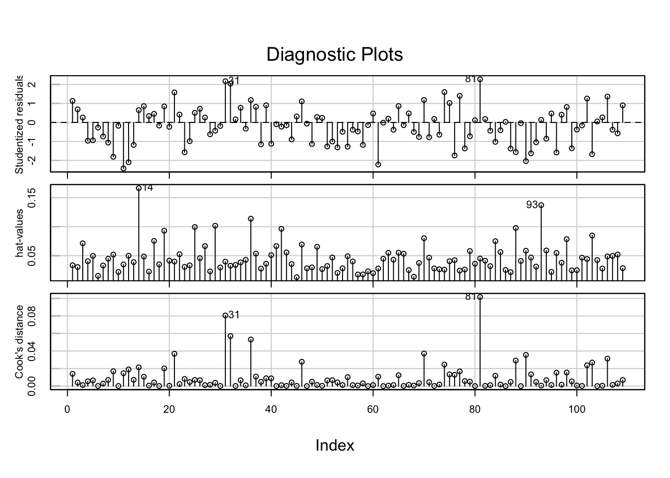
Examine Diagnostic Plots for Stepwise NB2 Model

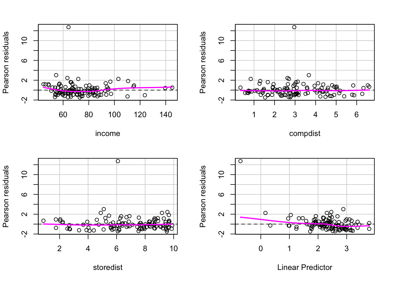
car::infIndexPlot(step.model.nb, vars=c("Studentized", "hat", "Cook"))

residualPlots(step.model.nb, tests = FALSE)

Examine Major Outlier

Store[which.max(residuals(step.model.nb, type = "pearson")),]

# A tibble: 1 × 7
  customers units income   age compdist storedist logunits
      <dbl> <dbl>  <dbl> <dbl>    <dbl>     <dbl>    <dbl>
1        10    19   64.2    22     2.96      6.09     2.94

Redoing Analysis w/ Outlier Removed

Store_sub <- Store[-11,]

m1_sub <- glm(customers ~ income + age + compdist + storedist, family = poisson(link = "log"), offset = logunits, data = Store_sub)

m2_sub <- glm.nb(customers ~ income + age + compdist + storedist + offset(logunits), link = "log", data = Store_sub)

m3_sub <- glm(customers ~ income + age + compdist + storedist, family = quasi(link = "log", var = "mu"), offset = logunits, data = Store_sub)

m4_sub <- glm(customers ~ income + age + compdist + storedist, family = quasi(link = "log", var = "mu^2"), offset = logunits, data = Store_sub)

Comparing \(X^2\) statistics with Outlier Removed

x_squared <- c(
    sum(residuals(m1_sub, type = "pearson")^2),
    sum(residuals(m2_sub, type = "pearson")^2),
    sum(residuals(m3_sub, type = "pearson")^2),
    sum(residuals(m4_sub, type = "pearson")^2)
  )
names(x_squared) <- c("Poisson", "NegBin", "Quasi(mu)", "Quasi(mu^2)")
dfs <- c(105,104,105,105)
x_squared

    Poisson      NegBin   Quasi(mu) Quasi(mu^2) 
  443.95875   110.23024   443.95875    38.63646 

pchisq(x_squared, dfs, lower.tail = FALSE)

     Poisson       NegBin    Quasi(mu)  Quasi(mu^2) 
3.140237e-43 3.192944e-01 3.140237e-43 1.000000e+00 

Examining QL(Var = mu^2) Model

QL(var = mu^2)

Looking at the plot of the residuals, it looks like this model may have underdispersion and is overestimating the variance in the data since almost all preds are within 1 sd of the actual value and all others fall within 2 sds

summary(m4_sub)

Call:
glm(formula = customers ~ income + age + compdist + storedist, 
    family = quasi(link = "log", var = "mu^2"), data = Store_sub, 
    offset = logunits)

Coefficients:
             Estimate Std. Error t value Pr(>|t|)    
(Intercept) -1.974864   0.463130  -4.264 4.43e-05 ***
income      -0.021256   0.003514  -6.049 2.33e-08 ***
age         -0.005001   0.003513  -1.423 0.157628    
compdist     0.175309   0.048876   3.587 0.000512 ***
storedist   -0.129983   0.033036  -3.935 0.000151 ***
---
Signif. codes:  0 '***' 0.001 '**' 0.01 '*' 0.05 '.' 0.1 ' ' 1

(Dispersion parameter for quasi family taken to be 0.3715045)

    Null deviance: 66.701  on 108  degrees of freedom
Residual deviance: 40.173  on 104  degrees of freedom
AIC: NA

Number of Fisher Scoring iterations: 6

infIndexPlot(m4_sub, vars = c("Studentized", "hat", "cook"))

residualPlot(m4_sub)

# residualPlots(m4_sub, tests = FALSE)

Continuing Analysis with NB2 Model

step.model.nb.sub <- step(m2_sub, scope = ~ .^3, k = 2, direction = "both", trace = 0)
summary(step.model.nb.sub)

Call:
glm.nb(formula = customers ~ income + compdist + storedist + 
    compdist:storedist + offset(logunits), data = Store_sub, 
    init.theta = 4.145108845, link = "log")

Coefficients:
                    Estimate Std. Error z value Pr(>|z|)    
(Intercept)        -1.445901   0.621089  -2.328  0.01991 *  
income             -0.019835   0.003542  -5.600 2.14e-08 ***
compdist           -0.005541   0.121957  -0.045  0.96376    
storedist          -0.237411   0.076925  -3.086  0.00203 ** 
compdist:storedist  0.025685   0.016511   1.556  0.11979    
---
Signif. codes:  0 '***' 0.001 '**' 0.01 '*' 0.05 '.' 0.1 ' ' 1

(Dispersion parameter for Negative Binomial(4.1451) family taken to be 1)

    Null deviance: 188.11  on 108  degrees of freedom
Residual deviance: 112.39  on 104  degrees of freedom
AIC: 694.86

Number of Fisher Scoring iterations: 1

              Theta:  4.145 
          Std. Err.:  0.772 

 2 x log-likelihood:  -682.862 

sum(residuals(step.model.nb.sub, type = "pearson")^2)

[1] 109.3899

Model VIFs

vif(step.model.nb.sub)

            income           compdist          storedist compdist:storedist 
          1.353989          10.565500          10.214381           8.089504 

Centering Predictors

Store_sub <- Store_sub %>%
  mutate(
    cage = scale(age, center = TRUE, scale = TRUE)[,1],  
    cincome = scale(income, center = TRUE, scale = TRUE)[,1],   
    cstoredist = scale(storedist, center = TRUE, scale = TRUE)[,1],
    ccompdist = scale(compdist, center = TRUE, scale = TRUE)[,1]
  )

nb.main.cent.sub <- glm.nb(customers ~ cage + cincome + cstoredist + ccompdist + offset(logunits), link = log, data = Store_sub)

step.nb.cent.sub <- step(nb.main.cent.sub, scope = ~ .^3, k = 2, direction = "both", trace = 0)
summary(step.nb.cent.sub)

Call:
glm.nb(formula = customers ~ cincome + cstoredist + ccompdist + 
    cstoredist:ccompdist + offset(logunits), data = Store_sub, 
    init.theta = 4.145108845, link = log)

Coefficients:
                     Estimate Std. Error z value Pr(>|z|)    
(Intercept)          -4.01366    0.06428 -62.442  < 2e-16 ***
cincome              -0.36879    0.06585  -5.600 2.14e-08 ***
cstoredist           -0.36482    0.08512  -4.286 1.82e-05 ***
ccompdist             0.25702    0.07210   3.565 0.000364 ***
cstoredist:ccompdist  0.08928    0.05739   1.556 0.119785    
---
Signif. codes:  0 '***' 0.001 '**' 0.01 '*' 0.05 '.' 0.1 ' ' 1

(Dispersion parameter for Negative Binomial(4.1451) family taken to be 1)

    Null deviance: 188.11  on 108  degrees of freedom
Residual deviance: 112.39  on 104  degrees of freedom
AIC: 694.86

Number of Fisher Scoring iterations: 1

              Theta:  4.145 
          Std. Err.:  0.772 

 2 x log-likelihood:  -682.862 

sum(residuals(step.nb.cent.sub, type = "pearson")^2)

[1] 109.3899

Check VIFs again

vif(step.nb.cent.sub)

             cincome           cstoredist            ccompdist 
            1.353989             2.363400             1.617399 
cstoredist:ccompdist 
            1.943570 

Final Model Hypothesis Testing

Final Model Hypothesis Testing

final_model <- step.nb.cent.sub
summary(final_model)

Call:
glm.nb(formula = customers ~ cincome + cstoredist + ccompdist + 
    cstoredist:ccompdist + offset(logunits), data = Store_sub, 
    init.theta = 4.145108845, link = log)

Coefficients:
                     Estimate Std. Error z value Pr(>|z|)    
(Intercept)          -4.01366    0.06428 -62.442  < 2e-16 ***
cincome              -0.36879    0.06585  -5.600 2.14e-08 ***
cstoredist           -0.36482    0.08512  -4.286 1.82e-05 ***
ccompdist             0.25702    0.07210   3.565 0.000364 ***
cstoredist:ccompdist  0.08928    0.05739   1.556 0.119785    
---
Signif. codes:  0 '***' 0.001 '**' 0.01 '*' 0.05 '.' 0.1 ' ' 1

(Dispersion parameter for Negative Binomial(4.1451) family taken to be 1)

    Null deviance: 188.11  on 108  degrees of freedom
Residual deviance: 112.39  on 104  degrees of freedom
AIC: 694.86

Number of Fisher Scoring iterations: 1

              Theta:  4.145 
          Std. Err.:  0.772 

 2 x log-likelihood:  -682.862 

Remove Non-Significant Interaction

final_model <- update(final_model, ~ . - cstoredist:ccompdist)
summary(final_model)

Call:
glm.nb(formula = customers ~ cincome + cstoredist + ccompdist + 
    offset(logunits), data = Store_sub, init.theta = 4.043382074, 
    link = log)

Coefficients:
            Estimate Std. Error z value Pr(>|z|)    
(Intercept) -4.05873    0.05722 -70.932  < 2e-16 ***
cincome     -0.38955    0.06476  -6.015 1.79e-09 ***
cstoredist  -0.29453    0.07308  -4.030 5.57e-05 ***
ccompdist    0.25454    0.07285   3.494 0.000476 ***
---
Signif. codes:  0 '***' 0.001 '**' 0.01 '*' 0.05 '.' 0.1 ' ' 1

(Dispersion parameter for Negative Binomial(4.0434) family taken to be 1)

    Null deviance: 184.94  on 108  degrees of freedom
Residual deviance: 112.99  on 105  degrees of freedom
AIC: 695.35

Number of Fisher Scoring iterations: 1

              Theta:  4.043 
          Std. Err.:  0.751 

 2 x log-likelihood:  -685.345 

Add Age?

m.add.age <- update(final_model, ~ . + age)
summary(m.add.age)

Call:
glm.nb(formula = customers ~ cincome + cstoredist + ccompdist + 
    age + offset(logunits), data = Store_sub, init.theta = 4.104191251, 
    link = log)

Coefficients:
             Estimate Std. Error z value Pr(>|z|)    
(Intercept) -3.942974   0.109552 -35.992  < 2e-16 ***
cincome     -0.393319   0.064280  -6.119 9.43e-10 ***
cstoredist  -0.299527   0.072805  -4.114 3.89e-05 ***
ccompdist    0.257888   0.072462   3.559 0.000372 ***
age         -0.004254   0.003410  -1.248 0.212212    
---
Signif. codes:  0 '***' 0.001 '**' 0.01 '*' 0.05 '.' 0.1 ' ' 1

(Dispersion parameter for Negative Binomial(4.1042) family taken to be 1)

    Null deviance: 186.84  on 108  degrees of freedom
Residual deviance: 112.61  on 104  degrees of freedom
AIC: 695.83

Number of Fisher Scoring iterations: 1

              Theta:  4.104 
          Std. Err.:  0.765 

 2 x log-likelihood:  -683.829 

Add Any Interactions?

all.int <- glm.nb(customers ~ (income + age + compdist + storedist)^2 + offset(logunits), data = Store_sub)
anova(final_model, all.int)

Likelihood ratio tests of Negative Binomial Models

Response: customers
                                                       Model    theta Resid. df
1        cincome + cstoredist + ccompdist + offset(logunits) 4.043382       105
2 (income + age + compdist + storedist)^2 + offset(logunits) 4.217364        98
     2 x log-lik.   Test    df LR stat.   Pr(Chi)
1       -685.3454                                
2       -680.8121 1 vs 2     7 4.533308 0.7167027

Add Higher Order Terms?

all.hot <- glm.nb(customers ~ poly(cincome, 2) + poly(cage,2) + poly(ccompdist,2) + poly(cstoredist, 2) + offset(logunits), data = Store_sub)
anova(final_model, all.hot)

Likelihood ratio tests of Negative Binomial Models

Response: customers
                                                                                           Model
1                                            cincome + cstoredist + ccompdist + offset(logunits)
2 poly(cincome, 2) + poly(cage, 2) + poly(ccompdist, 2) + poly(cstoredist, 2) + offset(logunits)
     theta Resid. df    2 x log-lik.   Test    df LR stat.   Pr(Chi)
1 4.043382       105       -685.3454                                
2 4.335951       100       -678.9555 1 vs 2     5 6.389932 0.2701036

Higher Order term for Income is close to being a significant predictor at a 5% overall significance level.

summary(glm.nb(customers ~ poly(cincome, 2) + ccompdist + cstoredist + offset(logunits), data = Store_sub))

Call:
glm.nb(formula = customers ~ poly(cincome, 2) + ccompdist + cstoredist + 
    offset(logunits), data = Store_sub, init.theta = 4.181236503, 
    link = log)

Coefficients:
                  Estimate Std. Error z value Pr(>|z|)    
(Intercept)       -4.06130    0.05657 -71.787  < 2e-16 ***
poly(cincome, 2)1 -4.01502    0.65342  -6.145 8.02e-10 ***
poly(cincome, 2)2  1.03056    0.57903   1.780 0.075109 .  
ccompdist          0.25186    0.07195   3.501 0.000464 ***
cstoredist        -0.29356    0.07233  -4.059 4.93e-05 ***
---
Signif. codes:  0 '***' 0.001 '**' 0.01 '*' 0.05 '.' 0.1 ' ' 1

(Dispersion parameter for Negative Binomial(4.1812) family taken to be 1)

    Null deviance: 189.22  on 108  degrees of freedom
Residual deviance: 112.49  on 104  degrees of freedom
AIC: 694.3

Number of Fisher Scoring iterations: 1

              Theta:  4.181 
          Std. Err.:  0.783 

 2 x log-likelihood:  -682.303 

Final Model Diagnostics

summary(final_model)

Call:
glm.nb(formula = customers ~ cincome + cstoredist + ccompdist + 
    offset(logunits), data = Store_sub, init.theta = 4.043382074, 
    link = log)

Coefficients:
            Estimate Std. Error z value Pr(>|z|)    
(Intercept) -4.05873    0.05722 -70.932  < 2e-16 ***
cincome     -0.38955    0.06476  -6.015 1.79e-09 ***
cstoredist  -0.29453    0.07308  -4.030 5.57e-05 ***
ccompdist    0.25454    0.07285   3.494 0.000476 ***
---
Signif. codes:  0 '***' 0.001 '**' 0.01 '*' 0.05 '.' 0.1 ' ' 1

(Dispersion parameter for Negative Binomial(4.0434) family taken to be 1)

    Null deviance: 184.94  on 108  degrees of freedom
Residual deviance: 112.99  on 105  degrees of freedom
AIC: 695.35

Number of Fisher Scoring iterations: 1

              Theta:  4.043 
          Std. Err.:  0.751 

 2 x log-likelihood:  -685.345 

vif(final_model)

   cincome cstoredist  ccompdist 
  1.286022   1.735287   1.652209 

Goodness of Fit Test

ts <- sum(residuals(final_model, type = "pearson")^2)
pchisq(ts, 104, lower.tail = FALSE)

[1] 0.2628477

# df = 109 - 5 (p includes estimate for gamma)

Check Expected Counts / fitted values to make sure Goodness of fit test is valid GOF test is good since no expected counts are below 1 and only 9% of counts are below 5.

exp_counts <- final_model$fitted.values

mean(exp_counts < 1)

[1] 0

mean(exp_counts < 5)

[1] 0.09174312

Leverage / Influence

n <- 109
p <- 5
high_leverage_cutoff <- 3*p/n
high_influence_cutoff <- qf(0.5, p, n-p)

c(high_leverage_cutoff, high_influence_cutoff)

[1] 0.1376147 0.8759709

There are no highly influential observations in the data

infIndexPlot(final_model, vars = c("hat", "cook"))

resid_plots <- residualPlots(final_model, smooth = FALSE, tests = FALSE)

attr(resid_plots, "dimnames")[[1]] <- c("Income (C)", "Distance to Store (C)", "Distance to Competitor (C)")
resid_plots

                           Test stat Pr(>|Test stat|)
Income (C)                  3.042815       0.08109516
Distance to Store (C)       1.159870       0.28149257
Distance to Competitor (C)  1.738773       0.18729438

Examine Obs with high leverage

These observations appear to be neighborhoods with high median income. Overall, these points are not influential so they will be kept in the model.

Store_sub[c(14, 93),]

# A tibble: 2 × 11
  customers units income   age compdist storedist logunits   cage cincome
      <dbl> <dbl>  <dbl> <dbl>    <dbl>     <dbl>    <dbl>  <dbl>   <dbl>
1         9  1113   145.     9     3.58      5.26     7.01 -1.10     3.83
2        14   966   140.    38     6.33      2.22     6.87  0.628    3.53
# ℹ 2 more variables: cstoredist <dbl>, ccompdist <dbl>

Outputting Final Model Predictions

units = Store_sub %>%
  summarize(mean = mean(units)) %>%
  unlist() %>% unname() %>% data.frame(units = .) %>% round(., digits = 0)

cincome = Store_sub %>%
  summarize(min = min(cincome), mean = mean(cincome), max = max(cincome)) %>%
  unlist() %>% unname() %>% data.frame(cincome = .) %>% round(., digits = 2)

ccompdist = Store_sub %>%
  summarize(min = min(ccompdist), mean = mean(ccompdist), max = max(ccompdist)) %>%
  unlist() %>% unname() %>% data.frame(ccompdist = .) %>% round(., digits = 2)

cstoredist = Store_sub %>%
  summarize(min = min(cstoredist), mean = mean(cstoredist), max = max(cstoredist)) %>%
  unlist() %>% unname() %>% data.frame(cstoredist = .) %>% round(., digits = 2)

pred_data <- crossing(units, cincome, ccompdist, cstoredist) %>%
  mutate(logunits = log(units))

pred_data %>%
  mutate(pred_count = predict(final_model, newdata = pred_data, type = "response")) %>%
  dplyr::select(-logunits) %>%
  mutate(pred_count = round(pred_count, digits = 3)) %>%
  arrange(desc(pred_count)) 

# A tibble: 27 × 5
   units cincome ccompdist cstoredist pred_count
   <dbl>   <dbl>     <dbl>      <dbl>      <dbl>
 1   654   -1.57      2.34      -2.59       81.0
 2   654   -1.57      0         -2.59       44.6
 3   654    0         2.34      -2.59       43.9
 4   654   -1.57      2.34       0          37.8
 5   654   -1.57     -1.81      -2.59       28.2
 6   654   -1.57      2.34       1.33       25.5
 7   654    0         0         -2.59       24.2
 8   654   -1.57      0          0          20.8
 9   654    0         2.34       0          20.5
10   654    0        -1.81      -2.59       15.3
# ℹ 17 more rows

# %>%
#   knitr::kable(format = "html")